The Blog

MHS helps multiple lab robots work in tandem to execute the experiment and troubleshoot errors.

Despite the availability of lab automation hardware, lab automation has remained largely off limits to models and researchers, outside of a small set of applications. Several technical barriers stand in between biology today and the development of an automated biology lab.

At Tetsuwan, our efforts to build such a lab have been focused on the development of better tools to interface researchers and agents with lab automation tooling via the development of automation. However, significant challenges remain in our ability to properly orchestrate a fleet of lab robots, varying in form factor and manufacturer.

In this blog post, we demonstrate the ability of HHMI Janelia Research Campus & Anthropic’s Model Hardware Standard (MHS) to help us overcome these challenges to contribute to a local citizen science project in Pacifica, California, and run a closed-loop experiment to optimize how our compiler makes decisions around pipetting settings.

You can find Anthropic’s blog on MHS, featuring this project and other interesting ones, at this link. For those of you coming from the MHS blog, more detail on the citizen science and heuristic optimization aspects of this project can be found in their respective sections. More detail about our work can be found across the other blogs published on this site.

Introduction to Lab Automation & ResearchOS

A wise man once wrote that most lab protocols can be automated, but few are worth automating. What does this mean? It means that despite the fact that we have had robots capable of performing experiments for decades, it seldom makes sense to invest the time and effort into automating a protocol.

Since the 1960s, labs have had automated machines that can pipette, de-cap, seal, shake, move labware, and perform most of the other functions of a biology lab. Yet the majority of biology experimentation remains manual. Part of the reason for this is that most biology experiments are fundamentally diverse; sample count, plate format, and the number of conditions change between runs as do the scientific parameters: dilution series depth, replicate count, incubation times, the number of timepoints, and so on.

Translating a single configuration into an automated workflow takes a specialist, known as an automation engineer, weeks to months. So, automation only pays off when an experiment configuration repeats at enormous scale, like in high-throughput screening, where one method runs across a library of hundreds of thousands of compounds. The bulk of experimentation, therefore, stays manual, inheriting all the potential errors and reproducibility problems that entails. Tetsuwan is building an automated biology lab, available to researchers and agents via an API. We believe that experimentation should be accessible, reproducible, and increasingly abstracted from researchers. Without addressing the problem detailed above, our lab would be confined to the limited capabilities of lab automation today, so we built ResearchOS to solve it.

ResearchOS is an automation platform that allows users to generate, run, and manage automated workflows without prior lab automation experience, within minutes. Claude works with users to turn natural-language protocols into a script written in our syntax for experiments, which is ultimately processed by a custom compiler into automation code.

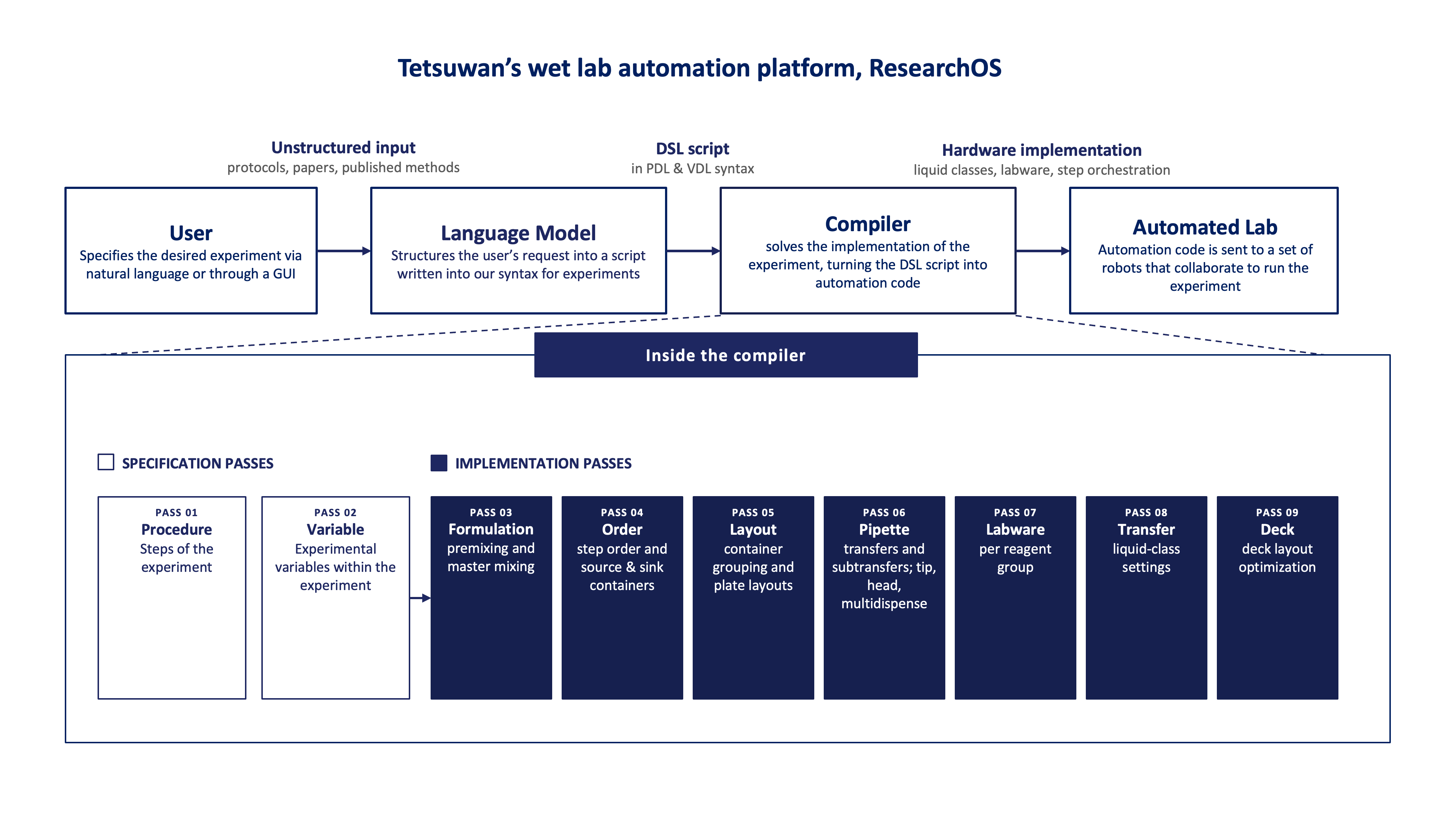
Built on top of a custom compiler, Tetsuwan’s ResearchOS bridges natural language to the execution of automated experiments.

In ResearchOS, a user describes the experiment at whatever level of abstraction they’re used to, and Claude resolves the ambiguities through dialogue before generating a program in our two domain-specific languages (DSLs), the Procedure Description Language and Variable Description Language.

The DSLs compile down through successive layers into the low-level instructions that a collection of lab robots can execute to perform the experiment. This makes the process simple, reliable, and inexpensive enough to justify the automation of one-off experiments.

Integrating the Model Hardware Standard (MHS)

ResearchOS is the API to the automated lab, but the lab itself presents a formidable orchestration challenge. It is, after all, a menagerie of pipetting robots, robotic arms, and automated labware that all use different languages and all have their quirks.

We implemented Model Hardware Standard (MHS) to allow us to use Claude as an orchestration layer over that fleet by allowing these devices to communicate with one another and with the user. With MHS, Claude can then catch errors in real time, optimize experiments, and coordinate with users.

Replacing our Scheduler with MHS

In our latest version of ResearchOS, we have fully replaced our scheduler and driver stack with MHS commands. In earlier iterations, our scheduler “Umataro” lived on an edge node co-located with the instrumentation. Umataro would read JSON payloads the compiler baked into the protocol and send HTTP or serial commands directly to a connected instrument.

Now, scheduling is handled by the Runs Coordinator in a container alongside the web application and the compiler. To enable MHS without official vendor support, we equipped each instrument with an SBC that acts as a connector.

Hardware Agnosticity

This orchestration layer allows protocols to stay hardware-independent. For example, a protocol might call for spinning a plate down at 15,000 × rpm for 5 minutes, for example, without naming a specific centrifuge.

ResearchOS uses MHS to query the network for a compatible centrifuge, learns its driver interface, and uses Claude to intelligently convert that force from the protocol into whatever the discovered machine accepts. For a machine that takes only rotor speed, that means dividing the force by the radius of the centrifuge’s rotor. The protocol author never even has to know which centrifuge they got, or how the measurement was converted.

Real-time Error Handling

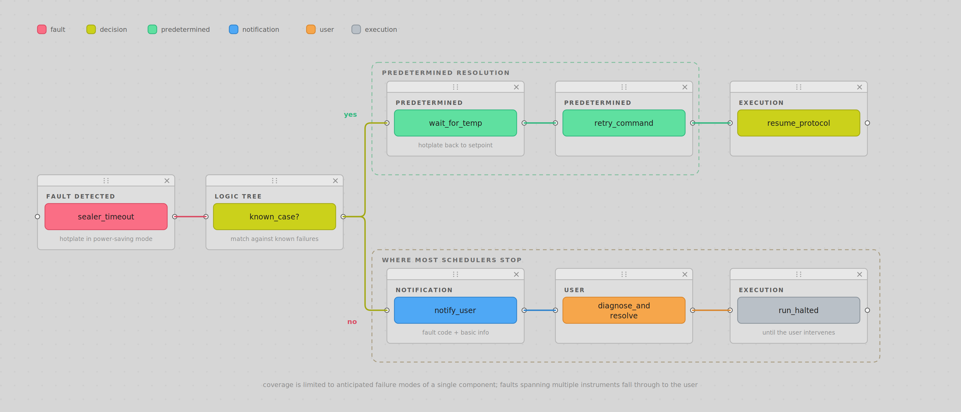
Implementing the MHS gave us the opportunity to extend scheduling capabilities to include error handling. Like many other schedulers, we can follow simple logic trees to determine if our system is in a known failure case and execute a predetermined resolution.

For example, plate sealer commands occasionally time out when the instrument enters a power-saving mode. In this state, the hotplate turns off and cools down, and it can take several minutes to return to temperature. The appropriate strategy is to wait until the hotplate returns to temperature, then retry the command. This is a very simple case, involving a single component of a single instrument with a known failure mode.

On an integrated system running a diverse set of experiments, one can expect a much broader range of issues involving multiple instruments. Most scheduling software stops here, prompting a human operator to come up with a resolution with a notification and some rudimentary information about the fault.

With MHS, LLMs like Claude can get information about the instrument's state, parameters, and capabilities, and understand the context. With this capability, the LLM can suggest an error-handling procedure to the operator via Slack and execute that program when authorized.

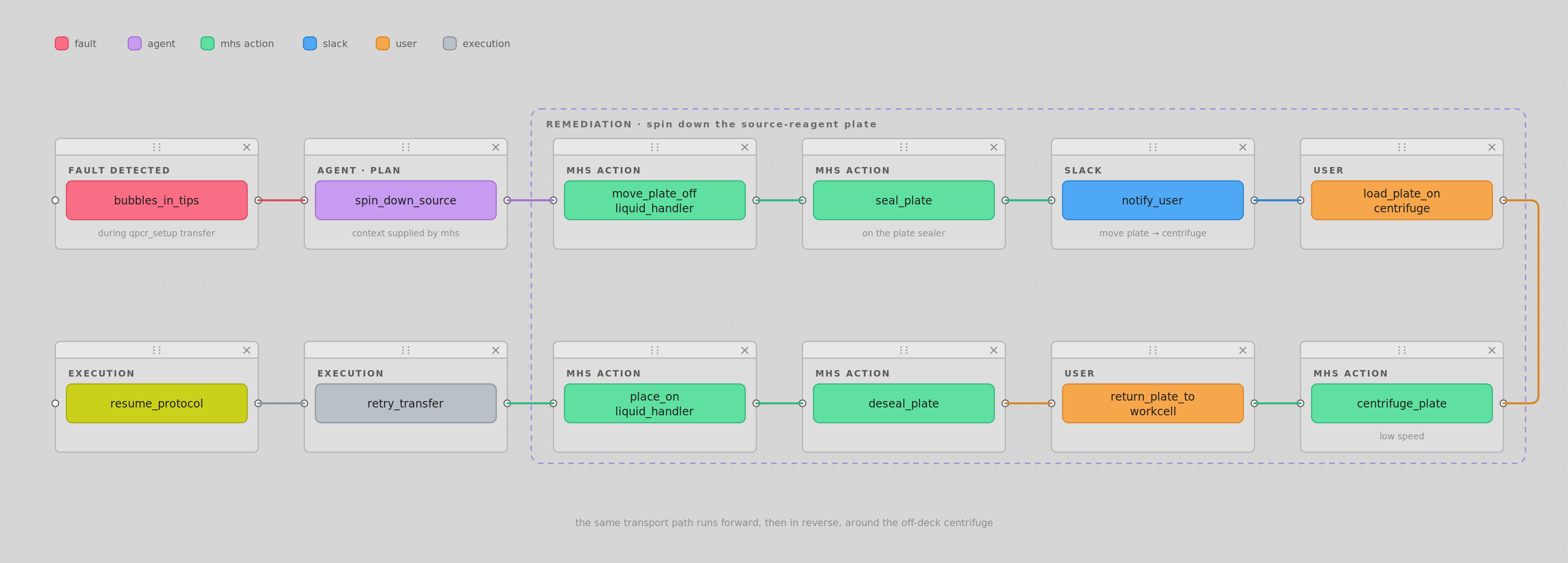
For example, as we were working on the qPCR setup protocol, the system noticed some bubbles in the tips as we were transferring reagents. The most likely cause of bubbles in the tips is insufficient source volumes or bubbles in the source.

MHS operates a camera to take pictures of each transfer, which is processed by a CV algorithm to identify pipetting behavior (such as bubbles and foam) to allow MHS to intervene upon the detection of error.

The LLM takes in this information, along with the capabilities of the instruments on the workcell and elsewhere in the lab. In this case, it suggests spinning down the plate containing the source reagent to remove any bubbles in that container. This triggers a series of MHS actions: moving the plate off the liquid handler, onto the sealer, and sealing the plate.

The human operator is prompted to move the sealed plate onto the off-deck centrifuge via Slack, at which point the agent again uses MHS to centrifuge the plate at a low speed. The process is repeated in reverse once the operator moves the plate back onto the workcell, desealing the plate, and placing it back on the liquid handler to retry the action.

Profiling Pollution in Pacifica’s San Pedro Creek

To test out our new MHS-enabled platform, we decided to visit Pacifica, California.

Floating in brisk water, looking back at shore, it is difficult to reconcile the fact that Pacifica’s Linda Mar Beach is only 25 minutes south of downtown San Francisco. Home to the famous “most scenic Taco Bell in the world”, Linda Mar is one of Northern California’s most beautiful beaches. It is also one of its most polluted.

For decades, the San Pedro Creek, which feeds into the Pacific at Linda Mar, has struggled with an unidentified source of fecal contamination. Though no smoking gun has been discovered, suspicion has fallen on horses, dogs, and aging sewer laterals.

The latter is what Dr. John Keener, Pacifica’s former mayor, thinks is most responsible for the pollution. Each house has a connection to the main sewer line created by a pipe called a sewer lateral. For many of the houses in Pacifica’s Linda Mar neighborhood, these pipes (called Orangeburg Pipes) are made of wood pulp.

Orangeburg pipes were popular during a steel shortage from 1940 to 1970, and most of Linda Mar was constructed in 1965. Predictably, the pulp pipes have not withstood the test of time as well as their steel counterparts. Keener hypothesizes that the aging sewer laterals are resulting in sewage leaking into the water table, which is collected by the stormwater system, and eventually dumped into the creek.

If Keener is correct, then the fecal contamination should be traceable back to mostly to humans (as opposed to dogs or horses, other sources of pollution). To test his hypothesis, Keener turned to a foundational molecular biology protocol, the polymerase chain reaction (PCR) to look for human-specific markers of pollution.

PCR copies DNA with nothing but a metal block (a “thermocycler”) that can heat up and cool down. DNA is a two-stranded molecule, and heating it separates the strands so they can be duplicated. Cooling it lets primers, which are short pieces of DNA that match the edges of the region you want copied, stick to those strands and mark where copying should start. Warming it back up, though not as much, lets an enzyme called a polymerase extend each primer along the strand it's stuck to, copying it.

A quantitative PCR (qPCR) adds a dye that glows brighter as copies accumulate, so we know how many copies there were to begin with. We can use this to measure how strongly a gene is switched on, to detect and quantify a pathogen in a patient sample, and to measure how much of a specific organism is present in an environmental sample such as creek water.

A screenshot taken from the “procedure” page, which shows users a graphical representation of their experiment after a protocol is uploaded. Shown above is the qPCR prep workflow used in this blog.

To contribute to the efforts of the San Pedro Watershed Coalition & Surfrider, we first decided to replicate the qPCR testing pipeline that Keener and his group had been contracting out to a lab in San Diego. We designed a panel to look for 8 species-specific markers and 2 general markers of bacterial contamination.

After some iteration on the design of the primers, we generated data that was consistent with Keener’s findings, suggesting that the majority of fecal contamination is originating from a human source.

With a proper primer set, our work over the coming weeks will focus on creating a higher-resolution map of contamination at and slightly upstream of the mouth of the creek, as well as profiling the Pedro Point neighborhood for the same fecal matter contamination that appears in San Pedro Creek. A future blog will be posted with data and results!

Closed Loop Compiler Optimization

One of our guiding theses at Tetsuwan is guaranteeing deterministic correctness. That means you will never have to test whether a generated automation script is doing the science you expected it to. You will never miss a column after asking an LLM to change the sample layout, you will never attempt to aspirate a negative volume because of a silent edit to the volume tracking logic, and you will never contaminate your sample because of lost context regarding a well’s content. Good abstraction should allow you to take these things for granted.

This guarantee is paramount in lab automation because validation in lab automation is hard. You can’t run a test script in milliseconds or open up a web app to check that your css rendered correctly. The most time-consuming (and expensive) part of automation engineering is testing it on a robot, tweaking it, and running it again.

So our compiler has to be deterministically correct. That means we have to define, according to the inputs, what is correctness and what is implementation quality (speed, cost, accuracy, waste).

As such, we design our compiler passes to first lower our intermediate representations into the correct model and then second a horizontal pass searches over candidate transformations. These transformations are a set of rewrite rules that provably preserve semantic meaning, guaranteeing correctness while giving us the flexibility to explore the implementation space. This strategy also makes incremental, interactive compilation safe. No poorly tuned heuristic or manual edit by a user can make a protocol wrong, only slower or less precise.

What are we optimizing?

The most common context for data collection and optimization in lab automation is liquid class optimization. This is the process of tuning pipetting parameters like flow rates, blow-out volumes, and air gaps to maximize accuracy and precision for each possible liquid type you might want to use. There are thousands of reagents and infinite mixtures of these reagents, so while there is a lot of data and best practices out there, a lot of time is still spent tuning this minutiae.

However, the type of liquid and the pipetting parameters you choose aren’t the only thing that affects accuracy! For example, you might use fast, imprecise liquid handling to plate fresh media onto your cells cultured in 6-well plates, but that would be entirely inappropriate when using the same media to create precise cell dilutions in 384-well plates for quantitative assays. Mastermixing, mixing order, tip type and head choice, multichanneling, multi-dispensing, source and destination labware types and their contents, and dead volume are all important contexts that can invalidate a liquid class choice.

Our compiler can collect this data at a granularity never before possible, with clean representations to learn about the implementation space and the relationships between these factors. This is how we tune our heuristics to continually optimize and improve our compiler.

The objective

If our objective is to maximize the quality of our implementations, we need to be able to calculate quality metrics. Some of these are easy, like counting how many tips or labwares are used or how much extra reagent is wasted. Others are trickier because we need a model that can predict what will physically happen on the robot. These are values like exact timing estimates, contamination risk, and predicted precision and accuracy.

The Opentrons Flex that we used for this experiment has a published manufacturer datasheet characterizing single dispenses of water in a fresh tip, but no data on multi-dispensing or over-aspiration. We used this data, along with our expertise and research on multi-dispensing behavior and compensation techniques, to inform the initial conditions for our hyperparameters.

Each of our multi-dispense candidates consists of a liquid, a tip on a pipette head, a per-dispense volume, a dispense count, and a compensatory over-aspiration volume. We can call the heuristic choices the compiler would naturally make the policy P and our error model that predicts the accuracy and precision of a given transfer M. The better M’s predictions are, the more informed choices P can make on tradeoffs, and the only way to improve M is by testing cells on a robot.

Even though protocols can have hundreds of transfers, most effects of a decision cell are local, so we can treat transfers as independent when testing their accuracy (bias) and precision (CV) while training our model M.

In this experiment, we expand the notion of testing how liquid classes affect accuracy and precision to testing how multi-dispensing affects accuracy and precision. The first step of this is improving our ability to predict a transfer’s accuracy and precision.

Designing the experiment

After isolating these components of pipette and transfer pass (liquid × tip × volume × dispense-count × over-aspiration), the raw space is enormous. So we eliminate based on feasibility (the aspiration draw has to fit into the tip - 221 million cells per liquid), deduplication (to weed out near-identical transfers by published CV, on a 2% grid - down to 337,000), and reasonableness (excessively large multi-dispense counts, large over-aspirate values, and small volumes in large tips). That leaves 55,877 cells per liquid, about 168,000 across our main three liquids tested.

We also generated a histogram of how frequently the compiler emits each transfer cell across realistic qPCR worklists. When we tune our compiler, we don’t simply want to fuzz all possible inputs and optimize metrics accordingly. It is important that our inputs are representative of real science so that we learn appropriate heuristics.

As mentioned, most of these choices only have local effects. However, because reagent waste, tips and tip boxes needed, tip economy, and number of tip swaps are calculated at the protocol level and couples every transfer to each other when we evaluate P the search is a joint search.

So we ran an experiment with our compiler: using the same qPCR procedure while sweeping sample count against primer count with m·n ≤ 768, forcing the compiler through cells both one-at-a-time and as sample joint policies. A PCR is roughly the simplest protocol there is, and yet we tested 22,330 protocols, 66 (m,n) points from 4 to 768 final reaction wells, 903 distinct decision cells over 6.03 million deliveries.

Some of the compiled protocols used tubes, some troughs, some reservoirs, plate layouts varied widely, some protocols were able to use multi-channeling others were not, some protocols were dominated by many small volume transfers, whereas others had quite a few large volume transfers, and there were at least 4 distinct mastermixing policies that were chosen across protocols. We ran this overnight for roughly eight hours and for each compilation we recorded reagent waste, step count, labware utilization, tip count, and tip-box utilization.

Some of the most interesting findings were in the cliffs created by sample and primer counts combos working well or poorly with multichanneling from stocks and mastermixes of different volumes to 96 well and 384 well plate layouts and the tradeoffs between reagent waste and transfer precision that mastermixing introduces. It also generated excellent data to indicate when a multi-dispense becomes “worth it” and what values of N are too small and which are too large to impact metrics like tip and time savings.

Executing the experiment

We dispensed a tartrazine tracer into plates under a controlled batch of cells and read absorbance through MHS on a Byonoy plate reader, which gives us delivered volume per well, and from that precision and accuracy per cell.

The campaign entailed 9,143 individual dispenses spanning 300 transfer types, with 1,508 measured conditions. On held-out sessions the learned model predicts dispense precision ~12% better than the datasheet, beating it on 33 of 45 held-out sessions, sign-test p ≈ 0.003, rising to ~17% on our highest-replication data.

The compiler sweep produced a frequency histogram of what transfer cells matter in qPCR protocols and how often they are generated, which helped to weigh what to measure next. Since robot time is a scarce resource and every experiment took 30 minutes to an hour and used up to four boxes of tips, we had to be very strategic about what to test on the liquid handler.

Each successive batch of experiments was chosen by the value of information for the current model of M, uncertainty weighted by frequency, weighted by whether the cell sat near a decision boundary where a change in M could flip P’s choice in the current pipette pass heuristics. Using this, Claude proposed the batch and more usefully was able to propose physics-based hypotheses to test.

Most of the effort of this project went into the experimental loop design rather than the model. Steps that we added to increase the experimental fidelity included:

• Taking several plate blanks and subtracting them out
• Deciding to prefill every well to a constant volume, which removes meniscus effects and makes absorbance depend only on dye mass rather than fill height (this is a tradeoff because in a real protocols the source and destination labwares might be empty or differently shaped)
• Masking missed wells or those with obvious bubbles
• Switching to carrying an in-plate reference standard so each plate self-calibrates to avoid evaporation and drift effects in the stocks
• Randomizing dispense order so that position on the plate stopped being perfectly aliased with position in the dispense sequence
• Increasing repetition, both within a plate and across sessions, because the effects we're chasing are small relative to how noisily a CV can be estimated from a handful of wells

On the model side, we started with manufacturing datasheet priors and some guesses based on the published physics and best practices of multi-dispensing. This added an N^2 term for the number of dispenses in a multi-dispense and treated over-aspirate relief like a starvation term that could offset error in the final dispense.

Every proposal was scored in a leave-one-run-out harness with bootstrapped confidence intervals, so an idea that the agent proposed had to generalize across whole sessions to count. As we accumulated more data the agent could propose changes to the shape of the model rather than just refitting coefficients leading to meaningful structural improvements to the model like splitting a term that was averaging two opposite effects and discovering that over-aspiration should scale with tip capacity rather than as an absolute volume.

The agent certainly still needed quite a bit of prodding intuition and correction at check in points and would occasionally struggle with reasoning about physical effects like evaporation. Additionally, tip supply and reagent refilling was only semi-unattended for these experiments, but as a starting point for dipping our toes into agentic closed loop optimization of our compiler we are very excited about this direction.

More accurately predicting accuracy and precision with M means a better policy P in our compiler, improving our heuristics permanently without ever sacrificing deterministic correctness.

Takeaways and future directions

In this initial data, we did not find most of the effects we expected. The multi-dispense penalty is very low, especially at large volumes and the over-aspiration benefit is marginal, and what exists is mostly concentrated at very small dispense volumes.

Interestingly, about a third of the CV we were measuring turned out to be plate-edge evaporation rather than pipetting effects. This is a well-understood effect, but we were surprised at how significantly the effect outpaced any signal from multi-dispensing or over-aspiration.